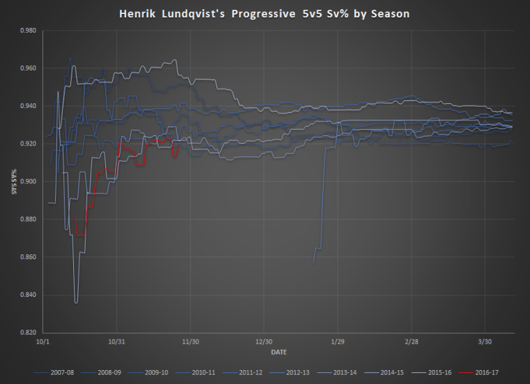
I looked at Lundqvist’s year-to-date stats back in late November and found that his play this year has been statistically weaker than every season since 2007-08 (which was the first season I could get the necessary data). I have added in the last five weeks of data and re-configured my graphs to make them a bit more reader friendly:
I looked at how Henrik Lundqvist’s play (a) has compared on a year-to-year basis and (b) how it tends to progress on a year-to-date basis. I used 5v5 Sv% and expected goals saved above average per 60 mins (xGSAA/60) as my two metrics. Both sets of data came from Corsica.
I chose 5v5 Sv% because it tends to eliminate a lot of team effects. All situations Sv% can be drastically affected by special teams based on the systems play that a team employs (as well as the efficacy at pulling it off). Overall, 5v5 Sv% tends to map decently year-to-year so it’s a good metric to look at as a measure of skill.
I chose xGSAA/60 because it helps address the issue of shot quality. xGSAA/60 basically looks at the types and distances of the shots taken and determines how many goals a hypothetical league average goalie would give up that night (ie, expected goals). By comparing this expected goals number against Lundqvist’s actual goals allowed number, we get an idea of how he performed against a league average baseline. The “per 60 mins” part helps to normalize for time in net. This stat is also only measuring 5v5 play.
I wanted to emphasize Lundqvist’s play this year against previous years as a composite so I chose colors that aren’t well differentiated for previous years (ie, 2007-16). However, if there is interest in having all of the years differentiated I can fulfill that request.
My observations:
Lundqvist isn’t doing well this year. His 5v5 Sv% is among the lowest of his career for this point in the season and his xGSAA/60 through yesterday is the worst of his career. There is some teeth to the idea that he is not playing at the same level as before.
His xGSAA/60 this year is very close to 0, suggesting that he is overall playing at a league average level during 5v5 play.
The idea that he is a slow starter is only true for the last few years. Earlier in his career he had solid starts to the season. There’s also a noticeable dip in almost every year for December, which is likely him cooling off from what looks like to be a lot of hot Novembers (just not this year).
His two best years by both stats appear to be 2015-16 and 2012-13. One year he received no votes for the Vezina while the other year he finished 2nd in voting. The Vezina voters really aren’t good at their job.
Honestly, I think it’s very fair to say we are seeing a below average performance from Hank relative to what we expect from him. This year he is facing a pretty normal mix of low-, medium-, and high-danger shots. It’s not like last year where the very high average shot quality he faced gave him average traditional stats and amazing underlying stats. Given the fact he’s coming off such a stellar season, I have a lot of hope that he can bounce back and play at a really high level this year.
However, going by the eye test I am at least a bit worried. There definitely have been games where he has let in total stinkers. And not just one stinker in one game, but a few stinkers in a few games each. But he still has long stretches where he plays solidly and makes great saves. Nonetheless, I would say there is not anything in particular that I see as an explanation for his poor play. No apparent injury or major changes in style of play. As far as I can tell, he’s more or less just playing more sloppy than usual.
Something I might investigate in the future is his progressive win threshold % (WT%) and loss threshold % (LT%). WT% is basically a measure of how often a goalie “steals games” and LT% measures how often they let in so many goals that the team in front is very unlikely to overcome it. Both are based on per game expected goals and goals against numbers. And at least for last year, he was absolutely elite by those numbers. One of the best in the NHL for both stats.
Per Cap Friendly, Lindholm’s new contract has a rather odd salary structure that may confuse a lot of people:
Year
Salary
2016-17
$3.00m
2017-18
$6.00m
2018-19
$6.75m
2019-20
$5.25m
2020-21
$3.75m
2021-22
$6.75m
We have generally grown accustomed to deals that are in some way flat, i.e., they may have a rising salary, uniform salary, or decreasing salary with term. And we have begun to grow used to either a salary drop in 2020-21 or an agreement that places most of that salary in signing bonuses. This latest tactic is “lockout-proofing” of contracts. So what gives with Lindholm’s tumultuous structure?
Variability Rules for Multi-Year SPCs
After all of the front-loaded deals helped set the 2012 lockout into motion, the Collective Bargaining Agreement (CBA), a labor contract between the NHL and the players’ union known as the NHLPA, came to include rules that were meant to eliminate such practices. One such set of rules is found in Section 50.7 of the CBA: Variability Rules for Multi-Year Standard Player Contracts (SPCs).
Paragraph 50.7(a) introduces the idea of “Front-Loaded SPCs.” Front-loaded SPCs are basically those aforementioned contracts that set the lockout in motion. A classic example is Marian Hossa’s contract:
Year
Salary
2009-10
$7.90m
2010-11
$7.90m
2011-12
$7.90m
2012-13
$7.90m
2013-14
$7.90m
2014-15
$7.90m
2015-16
$7.90m
2016-17
$4.00m
2017-18
$1.00m
2018-19
$1.00m
2019-20
$1.00m
2020-21
$1.00m
The original intention of these deals was to drive down the cap hit of the contracts by adding on low salary years at the end of the contract that the player would skip over by retiring. The 2012 CBA negotiations sought to eliminate these contracts by (a) limiting contracts to 8 years max and (b) introducing rules for how salaries can be structured on a year-to-year basis.
So paragraph 50.7(a) introduces the following limits on Front-Loaded SPCs:
Maximum of 35% change from year-to-year.
Maximum of 50% change from highest-salary year to lowest-salary year.
It’s pretty clear that the Hossa deal would violate this agreement if it were signed today. And it appears at first glance that the Lindholm contract does as well. After all:
It has a maximum year-to-year change of 50%, and
a maximum highest-salary to lowest-salary change of 56%.
Then why was this contract allowed to go through? Well, that lies in the definition of a Front-Loaded SPC. The following process for determining if a contract is a Front-Loaded SPC is spelled out in items 50.7(a)(i)(A)-(E) of the CBA:
Add up the total salary (including bonuses) of the first half of the contract. (Note: if there’s an odd number of years, take half of the “middle year.”)
Divide the combined salary of the first half of the contract and divide it by half the number of years of the contract.
Compare against the AAV of the full contract.
If the “first half average salary” is greater than the AAV, then you have a Front-Loaded SPC.
So let’s go through this process with Lindholm:
We know he has a 6-year contract with an AAV of $5.25m.
So adding up and averaging the first three years of his deal: $3.00m + $6.00m + $6.75m = $15.75m.
$15.75m / 3 yrs = $5.25m / yr
$5.25m / yr is not greater than the AAV ($5.25m), therefore this is not a Front-Loaded SPC.
Thusly, we need to refer to the next set of rules to see what actually governs the salary structure of Lindholm’s contract. Paragraph 50.7(b) applies to all non-Front-Loaded SPCs and states:
The difference in salary between the first two of the SPC cannot exceed the lower of those two salaries.
A year-to-year increase cannot be greater than the lower salary of the first two years of the contract.
A year-to-year decrease cannot be greater than 50% of the lower salary of the first two years of the contract.
Putting It All Together
It’s clear to see that there are many things going on with Lindholm’s contract here. To quote Walter Sobchak from The Big Lebowski, “It’s a Swiss fuckin’ watch.” Every single year is tangled with a requirement from at least one of the rules.
For starters, the first three years must sum up to no more than $15.75m in order to avoid having an average salary that does not exceed the AAV ($5.25m) of the entire contract.
Next, the first two years are specifically chosen to ensure that all of the year-to-year variability follows suit. The $3.0m and $6.0m salaries set the maximum year-to-year decrease at $1.5m (half the lower of the two salaries) and the maximum year-to-year increase at $3.0m (equal to the lower of the two salaries).
With the first two years set at a combined $9.0m, that means the third year must be $15.75m – $9.0m = $6.75m.
From there, the contract dips down as much as possible year-to-year for two years in order to create the lowest possible salary in the expected lockout year (2020-21). After two straight $1.5m decreases, the contract takes on salaries of $5.25m and $3.75m in the 4th and 5th seasons, respectively.
Finally, the last season is an attempt to have the highest possible salary, which leads to the maximum potential year-to-year increase of $3.0m. This puts the final season of the deal at $6.75m.
Relationship between different Year 1 salaries and their resultant Lockout Year salaries for Lindholm’s contract.
Every single year is optimized here. Increasing the value of the first two years results in less lockout protection, no matter how you try to arrange the salary structure within the rules. (E.g., I increased the first two years to $3.25m and $6.5m and ended up with $3.8m in the lockout year, which is $50k more than in the actual contract.) Similarly, dropping the values of the first two years will result in some exceedingly suboptimal salary structures. (E.g., I dropped the first two years to $2.75m and $5.5m, which resulted in a salary of $4.75m in the lockout year, which is not at all desired.)
Concluding Thoughts
So ultimately, we see a pretty interesting salary structure that at first glance appears funky. But after going through the applicable rules, we can see that each year is a carefully designed puzzle piece to fit this specific puzzle. Now remains only one question: Why not avoid all this nonsense by just committing all but $1m of his salary in the potenital lockout year to a signing bonus? That would have afforded more protection and without the funky contract numbers.
In this post I will evaluate this trade from the perspective of a New York Rangers fan. I plan to evaluate the following aspects of this trade:
Statistics-based performance review
Statistics-based usage review
Brief “eye test” statements
Contract, cap, and asset considerations
Concluding remarks
1. Statistics-Based Performance Review
Unless noted otherwise, all of the charts to follow were constructed using 2014-16 data for 5v5 situations with zone-, score-, and venue adjustments where applicable. The data has been sourced from Corsica. I will frequently use stats that say “/60”, which means the stat is adjusted to “per 60 minutes of time on ice.” This addresses any difference in time on ice by these players.
Here are some basic player data just to set the stage:
J.T. Miller became the first of four arbitration-bound New York Rangers to ink a deal. On July 13th, he signed a 2-yr, $2.75m AAV contract, leaving him just one year shy of UFA status. Many have proclaimed this contract is a steal for the Rangers, but I think it is right on point. I also believe it will provide a benchmark for many of the other players lined up for arbitration right now. Thus, I have used Miller’s contract to develop a simple cap hit prediction model for those other players.
I originally started researching and writing about the Cap Advantage Recapture Penalty (CARP) in relation to Shea Weber trade rumors last summer. It was pretty shortly thereafter that I started bandying about the phrase “Shea Weber is untradeable.” The liability of the potential CARP looming over a small market franchise like Nashville would be too great, especially considering the significant likelihood that Weber will decide not to play until he’s 41. But it happened and now I’m wrong about that. (Well, not about the CARP stuff so read on…)
(Just a quick note, my first, second, and third posts on this topic can be found at the links provided. I highly suggest giving them a read if you need some background info on what the CARP is and how it works.)
However, the exciting thing is that now everyone is talking about the CARP and want to learn more about it. I still cling to my viewpoint that the NHL has done no wrong in creating this cap mechanism. The Predators (a) chose to match the offer sheet, (b) were a party to the creation of the current CBA including the creation of the CARP, (c) chose not to buy him out with their compliance buyouts, and (d) chose to trade him with $24.5m of cap advantage sitting on their books. They made multiple conscious decisions to not limit their liability to this penalty. But, I can’t ignore the fact that others are right about how the NHL will not let a small market team, especially one that is such a major success story in their push to hockey-fy the South, be crippled with a penalty that could easily set the franchise back 5-7 years. Thirty other owner groups / GMs might say “tough nuggets” to them, but Bettman will certainly do what it takes to maintain 31 strong teams and markets in the league.
For at least the last two years, the idea has been floated around that the New York Rangers play two different games: one when Lundqvist is in the net and one when he isn’t. That idea goes on to posit that the New York Rangers who show up when Lundqvist is off the ice is a much better team. Those Rangers create more offense knowing that they can’t just grind out low scoring, one goal games, and they play a tighter defensive game knowing that the King can’t just bail them out when they misstep. Overall, they play a better game of hockey without their safety net.
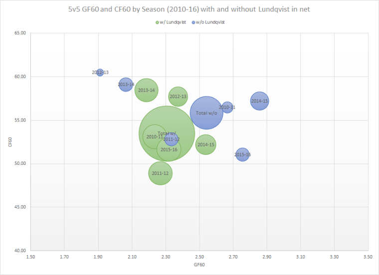
In this article I intend to begin looking into the notion that a team plays differently depending on who the goalie in net is. I will do so by examining something less directly tied to the goalie position. I will be looking at the GF60 and CF60 rates of three separate teams split based on whether their franchise goalie is in the net or not.
This idea isn’t without some cursory evidence. The Rangers were without Lundqvist for a sizable stretch in the 2014-15 season. A puck to the neck caused Hank to miss all of the Rangers’ games between Feb. 4th and March 26th, which was a 26-game stretch. Cam Talbot went on to shoulder much of the weight as the interim starter and ultimately he put up a great 0.926 performance. However, an early story line was the unexpected goal support from the Rangers for Talbot. From Feb. 10th to Feb. 22nd, the Rangers logged 33 goals in 7 games. And while they came back to earth shortly thereafter, the goal support still seemed to be there more for their goaltenders who aren’t named Hank. Talbot and MacKenzie stood in net for 38 games where the Rangers put up 3.04 GF60. Lundqvist received the slightly lower goal support of 2.89 GF60 over the course of 46 appearances. That came out to an extra 5.2% goals for Talbot and MacKenzie, which is an extra goal every 7 or so games.
Less Narrative, More Data and Graphs
I began by pulling 5v5 TOI, GF, and CF data for the New York Rangers’ goalies’ individual seasons from 2010-16, excluding 2012-13 (because the sample size is small for the lockout year). The data for guys besides Lundqvist were merged into a composite for each year.
The differences between the totals over these five seasons ended up being much larger than I expected. The Rangers scored an extra 0.23 GF60 in 5v5 play and generated 2.4 CF60 extra in 5v5 play when Lundqvist was on the bench or otherwise not playing. And in fact, the GF60 and CF60 data on a year-by-year basis was higher for the backups in 4 of the 5 seasons. The 5-year TOI totals were 16,202 min with Lundqvist and 5,758 min without. On a year-to-year basis, the TOI ranged from 2,225 to 3,088 min with Lundqvist and 743 to 1,785 min without. So the samples are decent in size.
Now, I do think this is compelling evidence that for some reason the Rangers are generally performing slightly better without Lundqvist in net. However, it is not possible to discern a reason from this data. Perhaps the players actually are more motivated to generate offense because they do not have their safety net. Perhaps the team’s coaches have made measurable changes to their personnel choices, such as decisions that are meant to try and keep the puck in the attacking zone. Perhaps the goalies themselves have significant contributions to the production, such as through stick handling.
To try and learn more about this apparent phenomenon, I investigated whether this situation has arisen on other teams. I chose to look at Nashville with Pekka Rinne and Chicago with Corey Crawford. Nashville, I thought, would provide a close parallel to the Rangers as both teams has generally been centered on an elite workhouse goaltender with a below average offensive team to support him. Chicago was to provide a stark contrast where I felt that Crawford was only depended upon to consistently deliver acceptable results and was infrequently leaned on to steal games. The Blackhawks tend to depend more on their offensive capabilities than the Rangers or Predators do, meaning that goaltending need not be as prized in Chicago.
The results were quite contrary to my expectations. The Predators, who seemingly would need to emphasize offense more without their star goaltender in net instead have mostly faltered in Rinne’s absence. Chicago, on the other hand, ramped up their production when they didn’t have their starter in net. It seems that the Blackhawks seek to capitalize more on their scoring opportunities to help support their backups.
Below is another look at the data. These graphs give direct year-by-year comparisons of the data for all three franchises with and without their starting goalie:
The GF60 data seems really noteworthy. For all three teams, 4 of the 5 dots fall on one side of the line. In the case of the Rangers and Blackhawks, they fall above the line, where offense is up when the starter is out. The Predators see a dip in production on all but one year when Rinne is off the ice.
The CF60 data mirrors the trend for the Rangers and Predators. However, the Blackhawks see their CF60 drop in 3 of the 5 years without Crawford in the net. This is starkly different than what was seen in the GF60 data.
Closing Statements
I intend to investigate this idea further with other teams that have had a consistent starter across the past six-year period (e.g., Pittsburgh, Los Angeles, Dallas, etc). I will avoid teams that have significantly switched their starters in that period to try and avoid adding yet another set of variables into this analysis. Even someone like Lehtonen will be pushing it as he has effectively gone from being the #1 goalie in Dallas to a 1A/1B goalie this past year.
I know the Rangers better than I do any other team in the league so they would be the best team for me to dig deeper on this matter. I have a suspicion that personnel choices by the coaches may be a significant driver of what was observed for the Rangers. However, failing that I can also look into “puck luck” in those games. It is possible that what we’re seeing is just an aberration by pure chance.
Ultimately I think something like this could be an important part of understanding how a major roster change could affect a team in indirect ways. There could be an argument made that moving Lundqvist for a slightly above goalie could be a better change than would be expected than just by the GA60 and salary cap impacts. There is evidence that that a slight GF60 bump could occur, which would in part mask a rise in GA60.
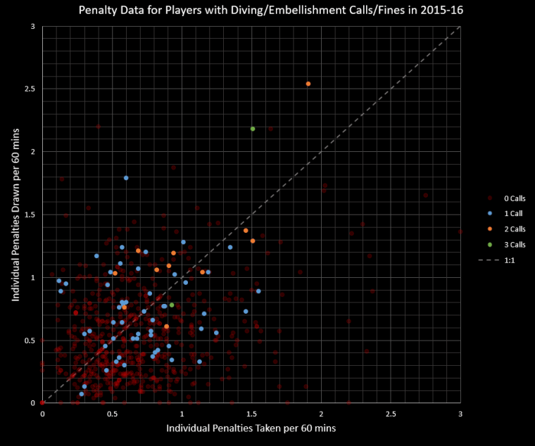
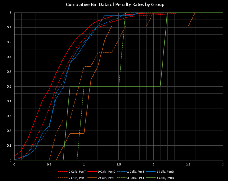
Thanks to the 2015-16 Diving/Embellishment List on Scouting the Refs and the easily accessible data on Corsica, I made a quick graph of how 5v5 player penalty rates break down depending on whether the player had either 0, 1, 2, or 3 diving/embellishment calls in 2015-16 or had been fined by the league for the same offenses.
The challenge was pretty simple. The 30 teams were the 30 active NHL franchises. (So someone who played for the Atlanta Thrashers would count as a Winnipeg Jet, etc.) I made it a personal rule to exclude WHA seasons so that means WHA-era Edmonton Oilers, Quebec Nordiques, etc., were out of the picture. Only NHL seasons with those franchises would count.
And when it became apparent that the challenge could not be answered favorably, I decided to figure out the maximum number of teams I could cover with different sized combinations of players. The results are as follows:
One Player – 12 Teams
This was an easy one. Most hockey fans know that Mike Sillinger is the king of the suitcase. Over his 17 season NHL career he played 1,049 games spread across 12 different teams. He was involved in 10 separate trades. He never spent more than 4 seasons with a single team (Detroit – although he only played 3 games in his inaugural season) and maxed out at 155 games with a single team (Columbus).
The next closest players have all played for 10 teams: JJ Daigneault, Jim Dowd, Olli Jokinen, Michel Petit, and Mathieu Schneider.
Two Players – 19 Teams
There are four such pairs of players in NHL history who have played for 19 different franchises between them. And all of these pairs share Mike Sillinger in common. His companions here are Jim Dowd, Bryan Marchment, Dominic Moore, and Lee Stempniak.
So the futures for Moore and Stempniak could see them moving their respective pair up to top spot in this category if they move on to the right team next year. Stempniak’s resurgence with the Devils and continued success with the Bruins should help him land a contract next year (at the tender age of 34). Moore, despite being 36 next year, could possibly find a new home. He still has a good reputation as a dependable fourth line center in this league.
Three Players – 25 Teams
Full size – The data table for players who played for 9+ NHL teams. (Carl Voss played for four teams that are now defunct.)
So the original challenge: 30 teams among 3 players. Can’t even get close. We top out at 25 teams in three separate trios. Even more shocking: The first one listed does not contain Mike Sillinger! Instead, they all share Grant Ledyard. Ledyard played 18 seasons in the league spread among 10 different teams. He did play five years each with Dallas and Buffalo in the middle of his career, but the bookends of his time in the league involved a lot of roaming. The trios were:
JJ Daigneult, Grant Ledyard, Bryan Marchment
Jim Dowd, Grant Ledyard, Mike Sillinger
Grant Ledyard, Bryan Marchment, Mike Sillinger
Ledyard probably ended up in all three lists because of the teams he played for. Among the 24 players who played for 9+ teams, it was most difficult to find players for Columbus (only 1 player), Buffalo (2 players), and Washington (3 players). Sillinger was great because he had played for Columbus, but a lot of his other destinations were places that had had 8+ other players play there. As a result, he was prone to “overlapping.” Ledyard played with Buffalo and Washington and played mostly for teams with 6 or less other “overlappers.”
Four Players – 29 Teams
This outcome totally sucks. With Carter Anson, Dominic Moore, Mike Sillinger, and Jarrod Skalde, I maxed out at only 29 teams! Why are you doing this to me Colorado? Fortunately Dominic Moore is still active so there is that teeny, tiny chance that this gets fixed next year, but I doubt it.
Calculating this with four players required me to move towards a programming solution. I did find a 25-team trio running through combinations in Excel, but I was not able to exhaust my search that way. And then I found a source that let me expand my pool to players with 8+ teams on their resumes, which put this all out of the reach of handwork.
I had a 54 player pool, which meant I would have to run through 316,251 different combinations. So I wrote a script in python to do it for me and keep track of the results. The frequency of the results can be found in the chart to the right. The data seems to be normally distributed with a mean of approximately 21.5. (Or maybe it’s more like a binomial distribution? I’m bad at stats so please correct me.) The range of the data is from 14 to 29.
Five Players – 30 Teams
As can be deduced from the previous section, you can easily find five players who, between them, have played on all 30 active franchises. There are literally hundreds of combinations stemming off the Anson + Moore + Sillinger + Skalde quartet above. And I would not be surprised to know there are hundreds or even thousands more that can be formed with any of the 54 quartets that cover 28 teams, the 509 quartets that cover 27 teams, etc.
Disclaimer
So it’s worth noting that the player pool I worked with only included those who had played for 8 or more NHL teams in their career. In the 54 player pool I used in my programmatic approach, I removed players with less than 8 teams due to defunct teams (e.g., Carl Voss) or from “doubled up” teams due to relocations (e.g., Hartford moving to Carolina).
I can confidently stand by my one player result for obvious reasons. My two player result cannot be beaten by a player with 7 or less teams to their credit, but it could possibly be tied. So both of those results as a maximum number will stand.
But I cannot rule out the possibility of there being higher results for three or four person combinations. A 7-team player and any of the four pairs that cover 19-teams could possibly form a 26-team trio. Similarly, Sillinger and two 7-team players could also reach 26. Similarly for quartets, there are a number of scenarios in which including 7-, 6-, or even 5-team players could lead to covering all 30 teams. And considering how much the player pool grows when going down as far as 5-teams, it becomes slightly plausible that a 30-team quartet does indeed exist.
So overall, I have an interest in adding 7-team player data to my set to determine what effect it might have on the results. I don’t see it being a challenge programmatically; the challenge seems to be finding an easy enough data source to work with. However, if I need to dive down into 6-team and 5-team data sets I might start encountering some challenges with my limited programming knowledge.Nonetheless, if any of you know where I might be able to come across helpful data sets, please let me know.
Brad Marchand, despite being one of the league’s biggest pests, is a highly skilled two-way winger who can play in all situations. He is both one of the best power play weapons for the Bruins and a key part of their penalty kill. So it is interesting to consider his prowess for getting calls and putting his team on the man advantage as well as for being called and sitting in the box while the Bruins play shorthanded. I plan to estimate the net “penalty effects” on the Bruins from Marchand’s penalty taking and drawing abilities.
Marchand and Penalties
Marchand has often been both the among the leading penalty takers and penalty drawers for the Bruins. His penalties taken (PF) numbers have been top three on the team in 2010-11 (3rd), 2013-14 (1st), 2014-15 (1st), and 2015-16 (t-1st). In the penalties drawn (PA) category, he has had top three finishes on the team in 2010-11 (1st), 2011-12 (1st), 2013-14 (2nd), 2014-15 (1st), and 2015-16 (1st). This has led to a large spread in how Marchand effects the amount of time that the Bruins special teams receive over the season: Continue reading “Penalty Effects: Brad Marchand and How He Effects the Bruins’ Special Teams Stats”→


