By @Chris_Beardy

J.T. Miller became the first of four arbitration-bound New York Rangers to ink a deal. On July 13th, he signed a 2-yr, $2.75m AAV contract, leaving him just one year shy of UFA status. Many have proclaimed this contract is a steal for the Rangers, but I think it is right on point. I also believe it will provide a benchmark for many of the other players lined up for arbitration right now. Thus, I have used Miller’s contract to develop a simple cap hit prediction model for those other players.

Miller is being paid at market value.

@HockeyStatMiner wrote a great article for Blueshirt Banter in May that predicted:

Here we have estimates of Hayes receiving a tad over $2.3 million, Kreider $3.6 million, and Miller a hair over $2.6 million. [emphasis my own]

Obviously he did some good work and produced a decently accurate estimate.

However, I think it can be refined. One issue I take with the above analysis is that it does not adjust cap hits for salary inflation. Ultimately, the Gagner, Ladd, and Oshie deals come out to $4.2m, $3.0m, and $3.0m in 2016-17 cap dollars, which averages to $3.4m. However, I would advocate removing Gagner’s contract from the mix. I strongly believe that Gagner’s 8-point night only 4 months below the negotiations over-inflated his value and/or Edmonton’s front office was largely incompetent when that deal was signed. So I’d put $3.0m as a fair value for Miller’s comparables.

Just as I felt Gagner over-inflated his value with an incredible 8 point night, I believe that Miller’s unrepeatable 9-goals-in-10-games hot streak over-inflated his value. I looked for comparables using Miller’s 72 “cold” games because I feel they are more representative of his production:

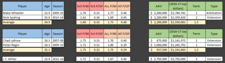
There seemed to be a “low risk / high ceiling” bracket and a “high risk / low ceiling” bracket, both of which had very different price points. Even after indexing the deals based on the growth of the cap ceiling, I found that a fair price for Miller was $2.55m, although I bet the Rangers could have used the LaRose and Regin contracts to knock him down to around $2.4m in arbitration.

Therefore, I find Miller’s contract to be reasonable for his level of skill displayed thus far and the expectations of his developmental ceiling. I believe that anything in between $2.4m and $3.0m was reasonable for him and the team based on these four production stats.

There are many comparable players awaiting arbitration.

Having established Miller’s contract as being a fair market price, I would like to turn the list of players currently awaiting their arbitration hearings. I have included both sets of Miller’s data on the table. Any savvy agent should argue that Miller’s stats were inflated from an incredible hot streak and would adjust his stats downwards similar to how I did. This would effectively set a higher price point for lower production numbers, which helps players earn more. Conversely, a savvy GM should be looking to pin as little money on as much production as possible, causing him to love the hot-streak-inflated numbers. Thus, both sets of numbers could be relevant to contract negotiations.

I created a simple prediction model from the data. I found the average of Miller’s two sets of stats and then calculated the relative difference of each players’ stats from Miller’s averaged stats. I then average these relative differences for each player. Next I raised each player’s average relative difference by an exponential coefficient that is meant to represent the premium paid for higher skilled players. Finally, I multiplied Miller’s $2.65m AAV by each player’s adjusted relative difference to reach their expected salary.

To give a concrete example, let us look at Mike Hoffman.

His relative differences to Miller’s averaged stats were 122%, 134%, 131%, and 162%. Together, these averaged out to 137%, which was Hoffman’s measure of production relative to Miller. Next, I had to find an exponential coefficient to represent the premium that Hoffman would fetch for being the best player in the group. To do this, I set my equation up for Miller’s stats with the streak and his stats without the streak. I used $3.0m AAV for the streak stats and $2.4m AAV for streak-less stats. I used Solver in Excel to find the coefficient at which the difference between the expected salaries and model salaries was least. (It turned out to be 1.27.) Then I plugged in Hoffman’s data to the equation to get my prediction.

My model is overly simplistic, but it’s a start.

Ultimately, I am excited to see how this model holds up. Obviously it is overly simplistic and will probably need some fine tuning. It doesn’t account for a lot of things:

• length of contract
• age of player (and years of remaining RFA)
• defensive contributions
• position premiums
• extra roles played
• pretty much everything else

But I am hoping to get a few 1-2 year deals that can help determine how accurate this model may be. Even if it’s wrong, new data will help illuminate where it’s wrong and how it might be improved.